Connect geometry
Reference closed building masses or meshes and connect them directly to Geometry.
Rhino 8 / Grasshopper
AeroField computes a three-dimensional exterior wind field around building geometry and turns it into clear, design-facing visualizations for early architectural comparison.
Three-dimensional exterior flow analysis
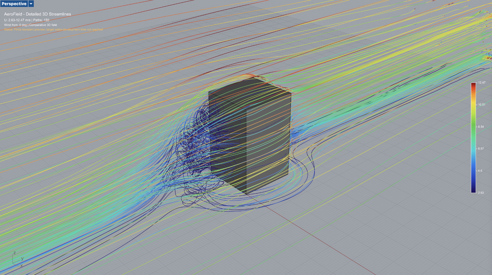
AeroField computes a three-dimensional exterior velocity field around one or more building masses. The resulting field can be examined for approach flow, acceleration, vertical deflection, wake formation, recirculation, shelter, and downstream recovery.
The numerical model is integrated directly into Rhino 8 and Grasshopper so that geometry, boundary conditions, field calculation, derived quantities, and visualization remain within the architectural design environment.
Study configuration
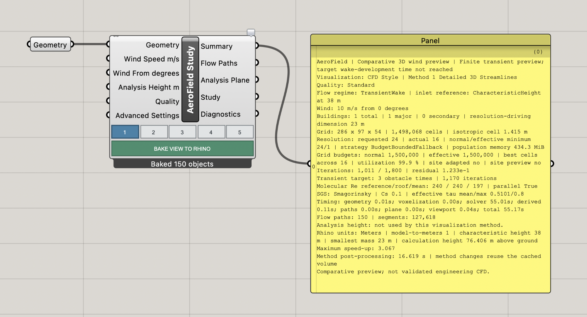
A standard study needs only a Geometry parameter connected to AeroField Study. Wind speed, direction, analysis height, and quality all have useful defaults and can be overridden when needed.
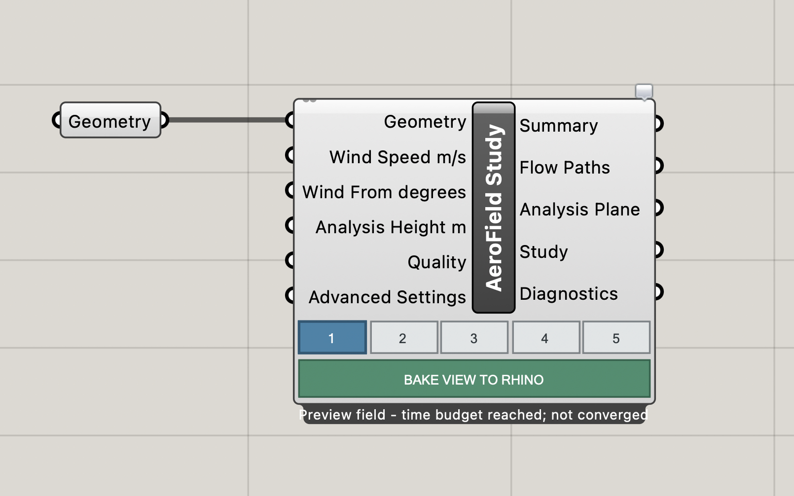
Reference closed building masses or meshes and connect them directly to Geometry.
Adjust wind speed, meteorological incoming direction, analysis height, or quality only when the defaults need to change.
Buttons 1–5 reuse the computed field to move between streamlines, wake, pedestrian map, sections, and surface exposure.
Computational framework
Study handles ordinary analysis. Numerical and domain controls exposes resolution, domain, wind profile, scalar, and display controls. Flow-field animation turns the current study into presentation-ready motion.
Field visualization
Each visualization samples or derives information from the same calculated three-dimensional field, allowing different physical characteristics to be examined without unnecessarily repeating the primary calculation.
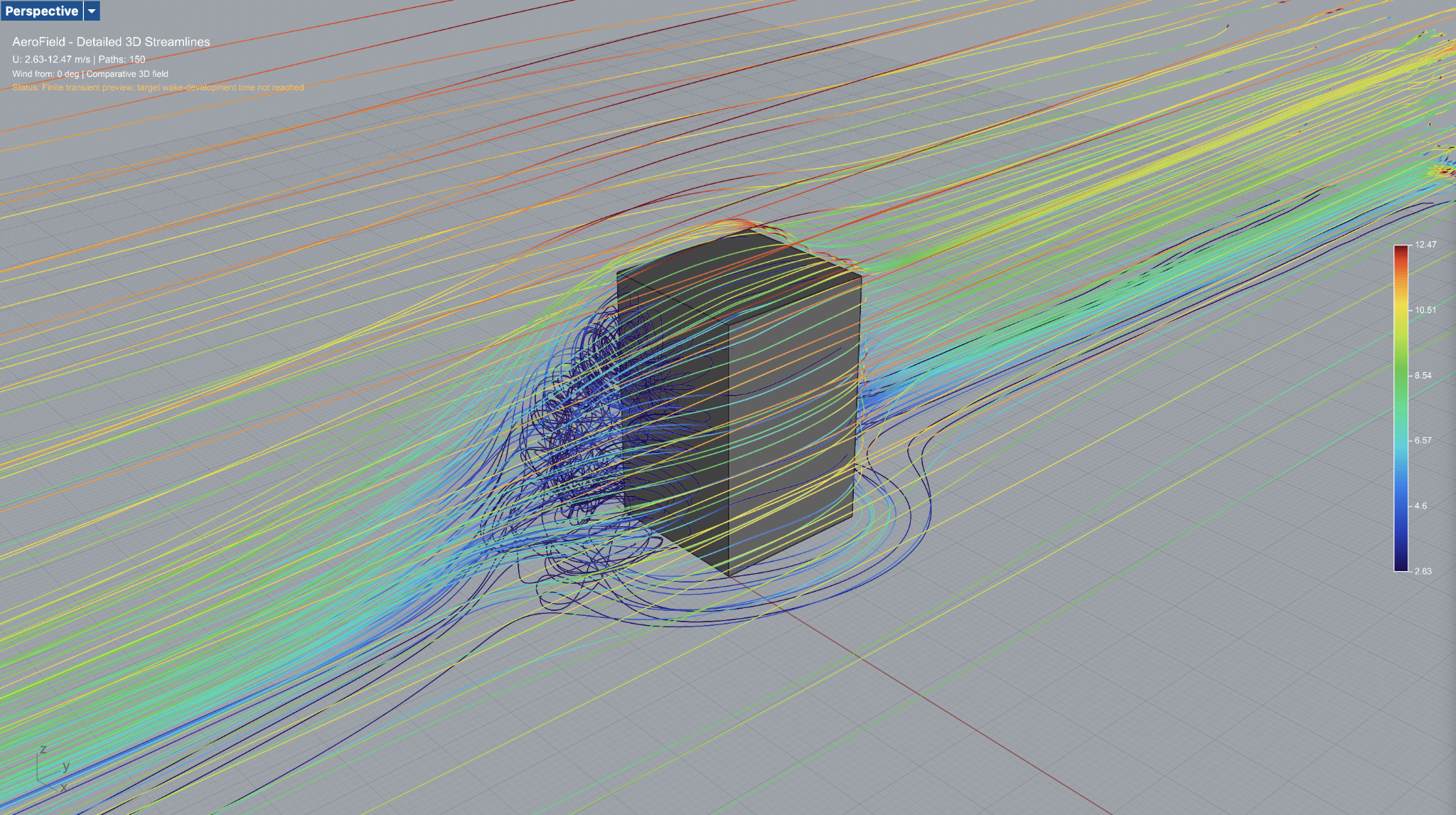
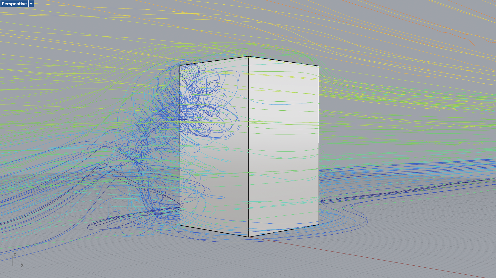
Detailed 3D Streamlines
Dense three-dimensional streamline families reveal approach flow, roof bypass, side deflection, downstream recovery, and local recirculation. Path color represents local velocity magnitude.
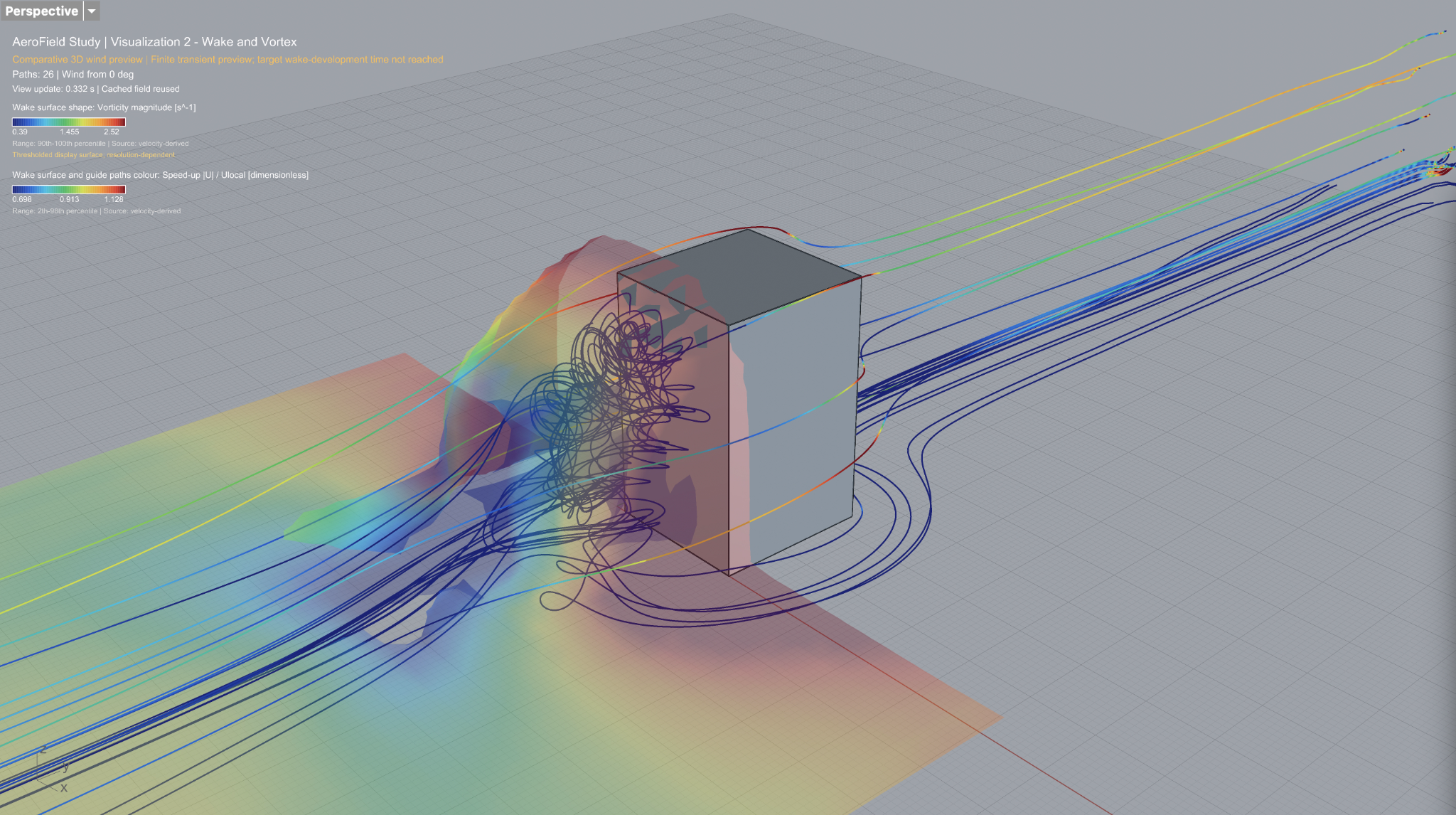
Wake & Vortex
Wake-oriented surfaces and guide paths make turning, shelter, and rotational structure easier to compare between design options.
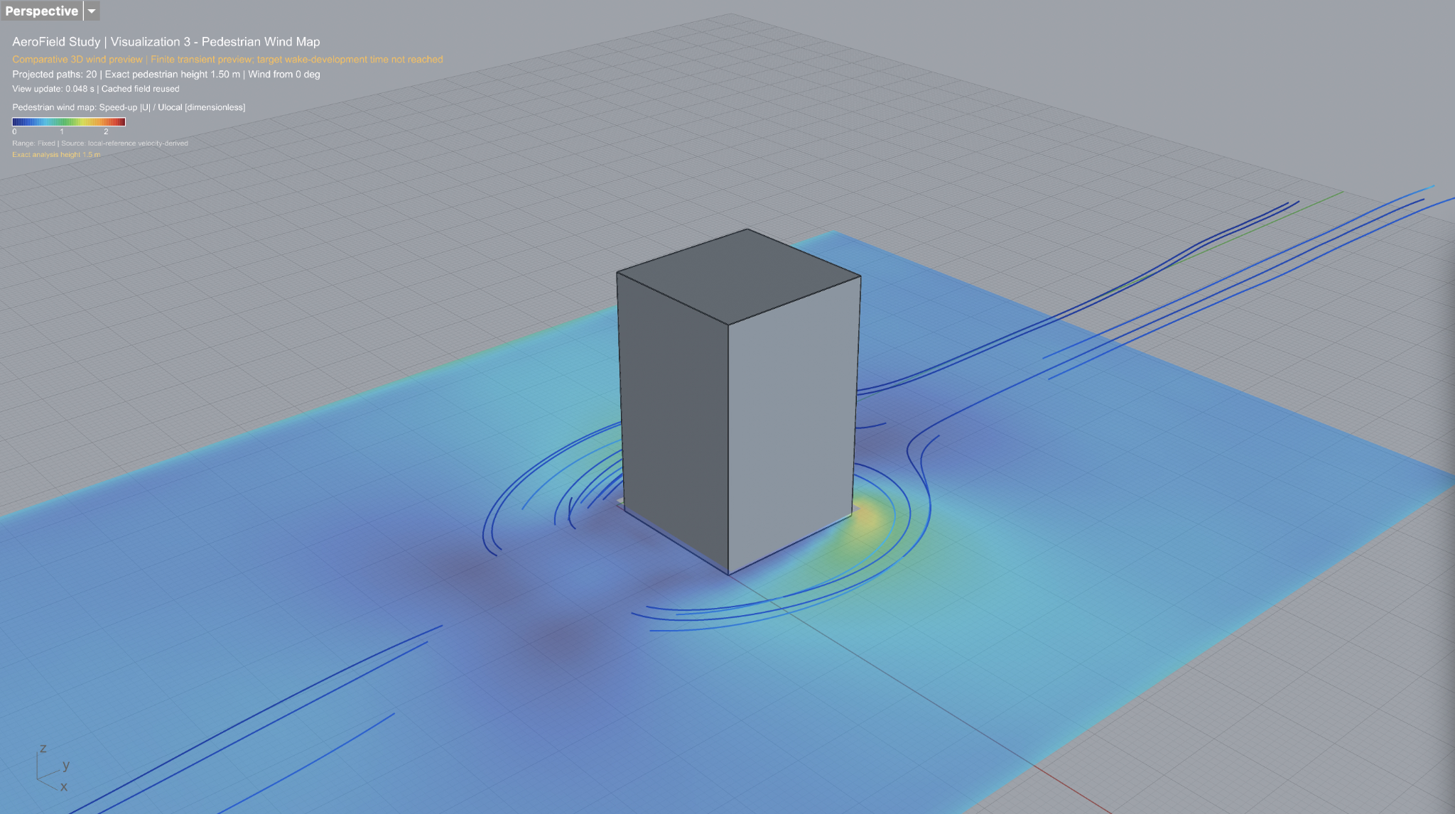
Pedestrian Wind Map
A horizontal analysis plane samples the stored field at the selected height. The default Speed-Up view compares local velocity with the undisturbed incoming wind at the same elevation.
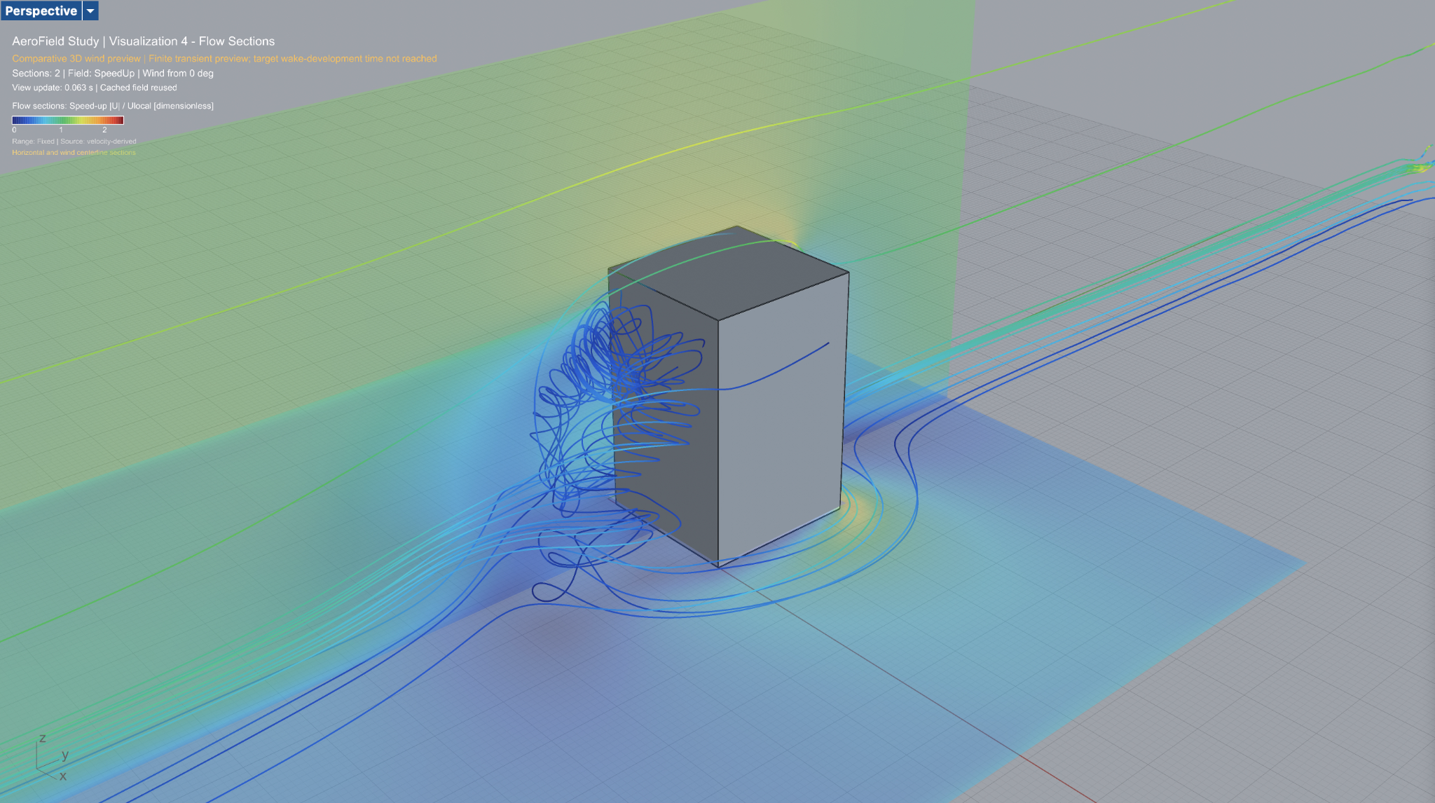
Flow Sections
Horizontal and vertical sections reveal scalar patterns that can be difficult to read in a dense three-dimensional path view, including Speed-Up, Speed, Pressure Proxy, Vorticity, Q Criterion, vertical velocity, and more.
Surface Exposure
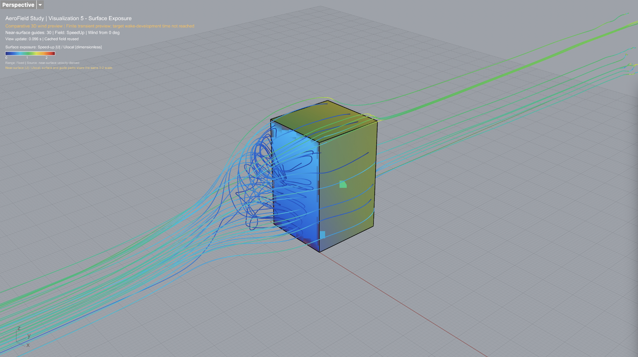
Color building façades and roofs by Speed-Up, Speed, or Pressure Proxy to see where geometry is comparatively more exposed or sheltered.
Numerical model
AeroField numerically evolves a three-dimensional velocity field on a discretized exterior domain around the input geometry. From that field it derives velocity magnitude, speed-up ratio, pressure proxy, vorticity, Q criterion, divergence, flow disturbance, speed deficit, and geometry-based visualizations.
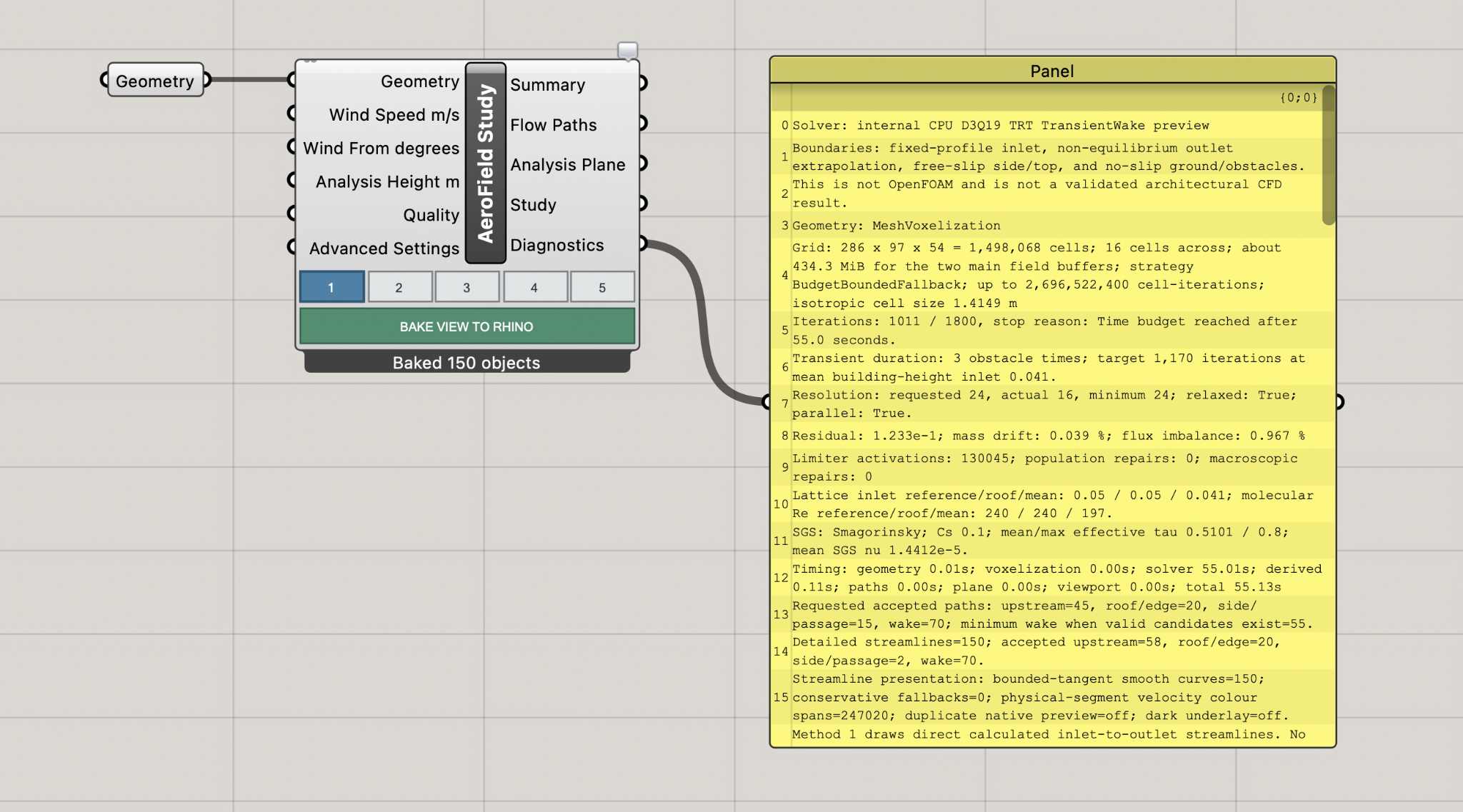
The current solver uses an internal CPU D3Q19 TRT transient-flow formulation on a voxelized three-dimensional domain, with Smagorinsky subgrid-scale treatment reported in Diagnostics. Summary and Diagnostics expose grid dimensions, achieved resolution, cell count, iterations, residuals, timing, boundary treatment, and field-generation status so the visualization remains traceable to its numerical setup.
Numerical and domain controls
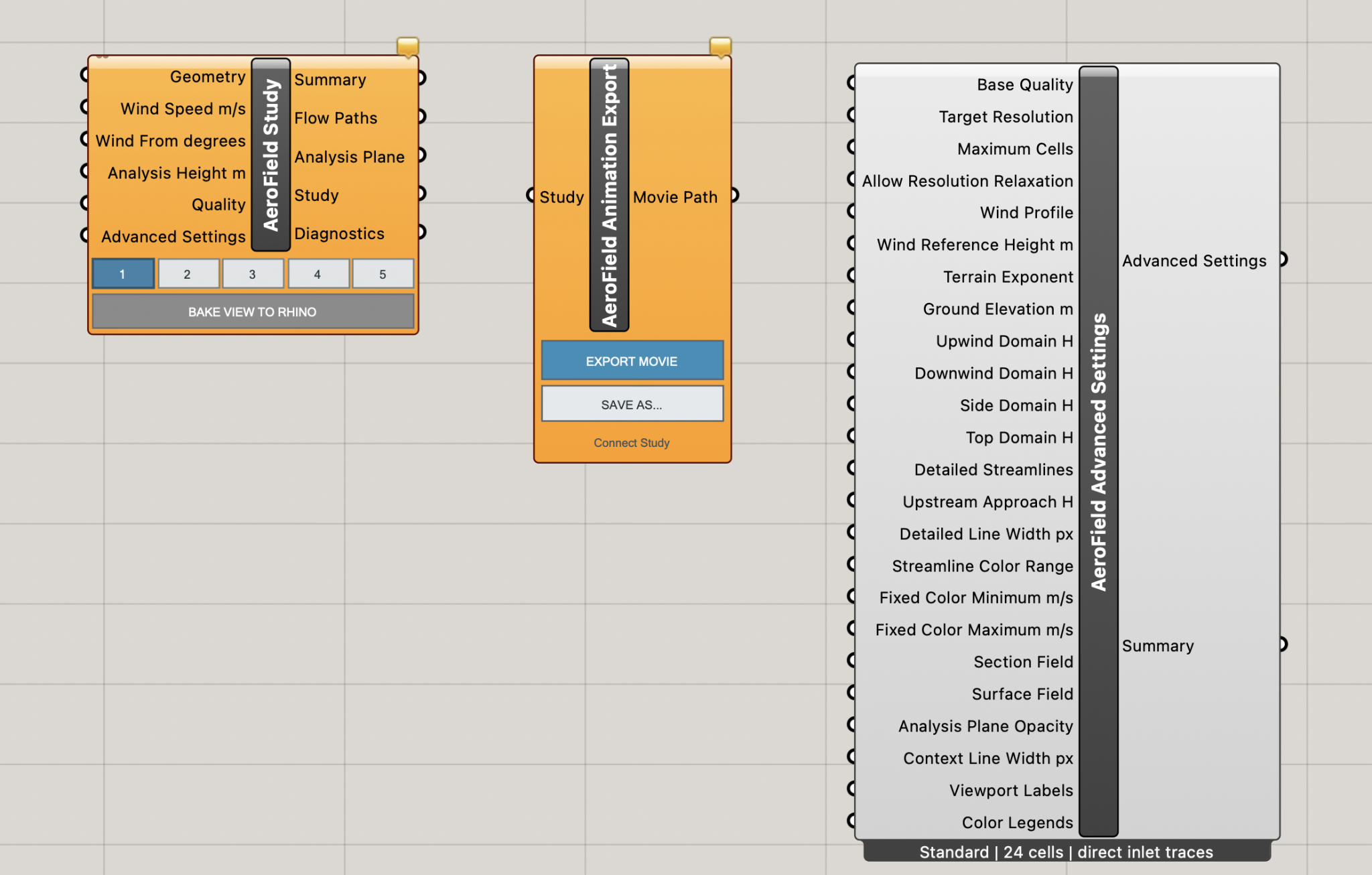
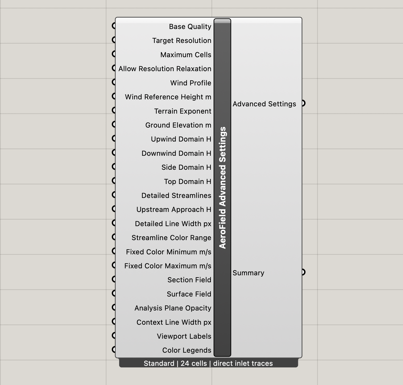
Numerical and domain controls is optional. When connected, it gives direct control over resolution, maximum cells, incoming wind profile, ground elevation, domain extents, streamline density, color range, scalar fields, line widths, opacity, labels, and legends.
Flow-field animation
Connect the Study output to Flow-field animation and AeroField prepares clean Full HD frames from the active Rhino camera. Export uses locally available formats through ffmpeg.
Geometry export
BAKE VIEW TO RHINO converts the active visualization into Rhino objects for documentation, diagrams, boards, rendering, and presentation. Flow Paths can also be baked through standard Grasshopper tools when only curves are needed.
Technical documentation
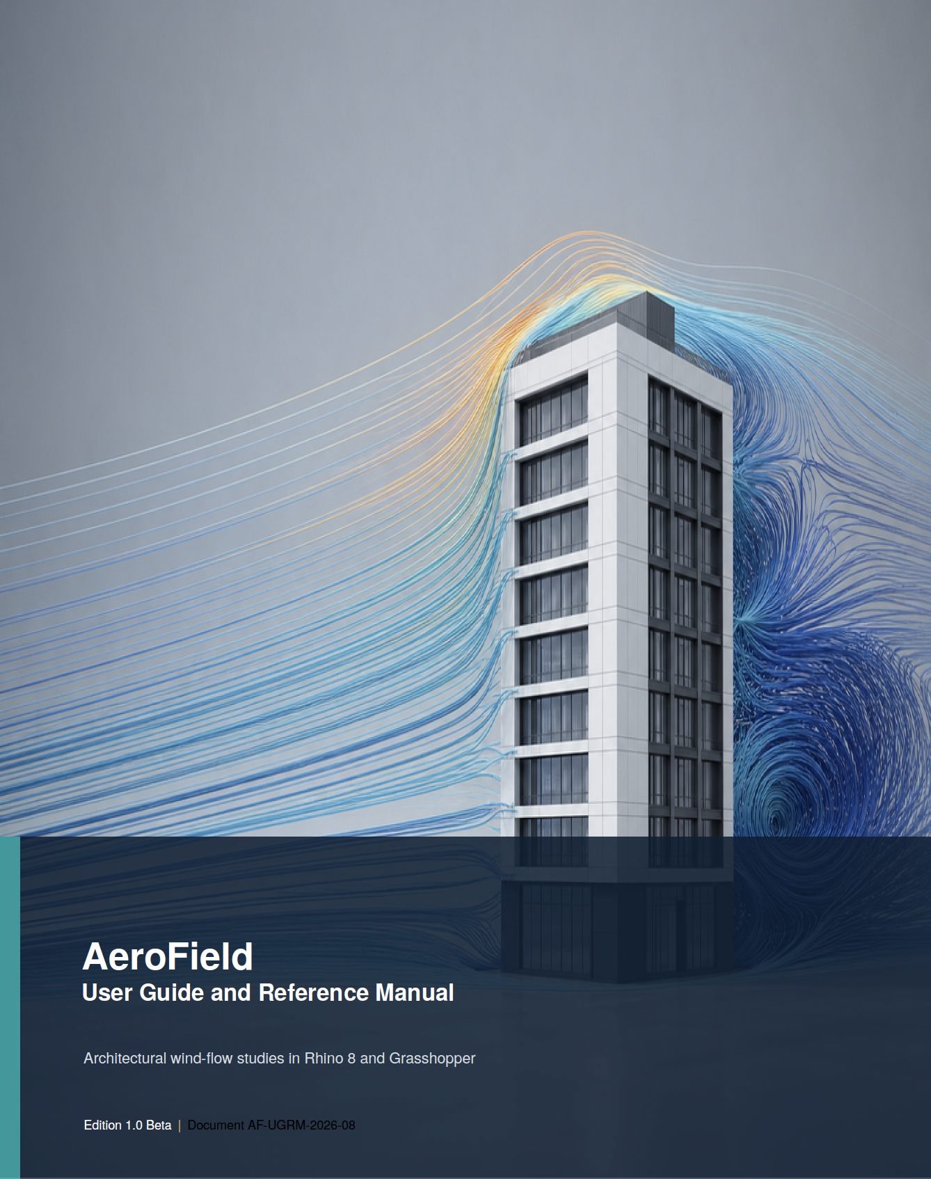
The AeroField manual covers installation, quick start, every public component, the five visualization methods, advanced settings, flow physics, scalar fields, baking, animation export, troubleshooting, recommended workflows, and interpretation limits.

Founder
AeroField began as a computational design project focused on making sophisticated environmental analysis more accessible within the architectural design workflow. It is developed as a free tool for the design community.
Founder & Lead Developer
Validation and scope
AeroField is not a substitute for validated engineering CFD, wind-tunnel testing, structural wind-load analysis, façade design pressures, pedestrian comfort certification, code compliance, or life-safety engineering. It is intended to help compare options, identify patterns, and decide where higher-fidelity specialist analysis is warranted.
Public beta release
For Rhino 8.30 or newer on macOS and Windows. Download the current public release, platform packages, and installation information from Food4Rhino.